Author: Ilina Yusra
One of the key questions that reservoir engineers come across in their work is how to determine the minimum number of grid blocks required in a reservoir model. Whether it is a full-field model or a simpler model, determining the number of grid blocks needed is not necessarily trivial, and failing in the choice of a number of grid blocks may result in a misleading result or longer CPU run times than needed.
One of the basics of reservoir simulation is the finite-difference formulation. It discretizes the spatial segmentation of the model into smaller parts, so-called grid blocks. By using Taylor series expansion, the error term (or sometimes known as discretization error) is second-order proportional to the grid block size (Δx2). In other words, the smaller the grid blocks the smaller the error.
Reducing the error is what one should aim for, in such case, all one needs to do is to use as many grid blocks as possible. However, the CPU time can increase significantly with the larger number of grid blocks. Imagine if the simulation took days, then increasing grid blocks might cost weeks if not months to finish. Then how do we find the optimum grid blocks number that can counterbalance smaller error and faster CPU time?
Our approach to find the optimum number of grid blocks is as follows:
- Start with a complete input dataset of the model. It is important to make sure that these not-grid-related inputs do not change during the gridding sensitivity.
- Choose the “starting” number of grid blocks along x-, y- and z-direction (Nx, Ny, Nz) arbitrarily based on experience and/or requirements for the particular process being simulated (e.g. depletion, EOR, both depletion, and EOR).
- Run the simulation one time. This will be the starting point for the gridding sensitivity (base case).
- Run a new case where Nx is increased while Ny and Nz are kept the same. Compare the results with the base case.
- Keep increasing Nx until the results “converge”, i.e. little “line-thickness” change in the reservoir model performance is seen with an increasing number of grid blocks. The minimum number of grid blocks needed to reach convergence will be the optimal Nx.
- Repeat steps 4 and 5 for Ny and Nz, respectively.
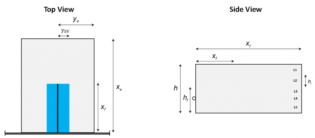
We will show you a simple exercise doing the gridding sensitivity. A one-dimensional homogeneous problem with 10 ft length, 2 ft width and 40 ft thick is carried out to model a reservoir oil system in a tight (nano-darcy) unconventional. The initial reservoir pressure is 6500 psia and reservoir temperature is set to 213o F. A producer well is located in the middle of the model and production is constrained by a minimum flowing bottomhole pressure of 1000 psia. The simulation is run for 100 days of primary depletion. To begin, Nx was set to 4, then Nx was increased until the results converge. The results are portrayed in the figures below.
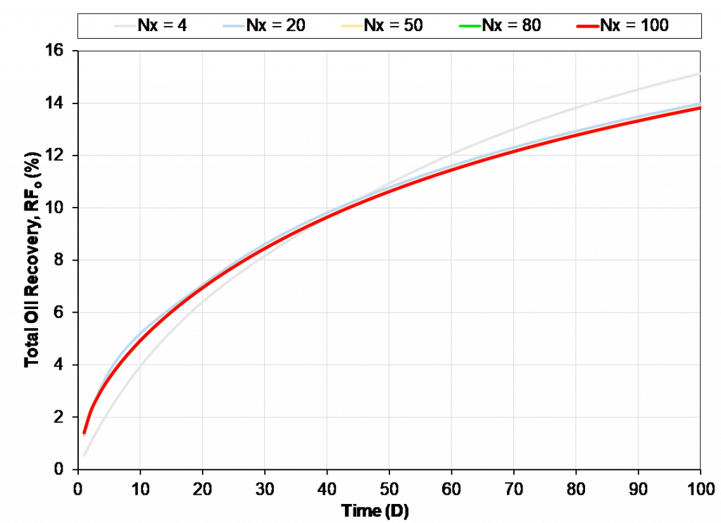
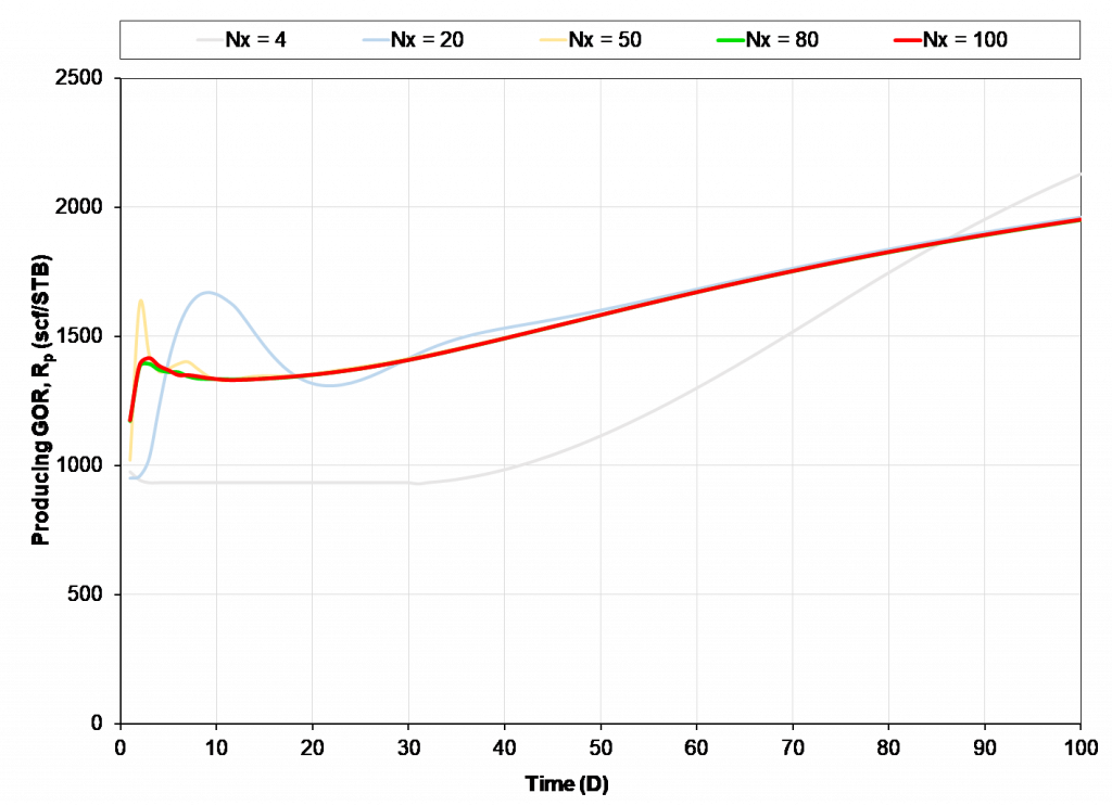
As the number of grid blocks in x-direction increases, the results start to converge to a single solution. The pressure and oil recovery from Nx=80 (green line) and Nx=100 (red line) are practically within line thickness. Moving forward Nx=80 can be used as “optimal”. From the results, the model with fewer Nx than the minimum needed predicts a “better” performance for the reservoir, while in fact the actual results are camouflaged by poor gridding.
However, as one studies more complex behavior such as early-time GOR development, RTA/PTA applications (with small-time requirements being important), or gas Huff-n-Puff EOR, further assessment of grid sensitivity may be made necessary, resulting in a larger number of grid blocks to provide a converged solution. Grid sensitivity can be a strong function of the process being modeled. Furthermore, the results can vary with the non-grid related input data – e.g. initial fluid system.
The grid size spacing can also impact the number of grids required to achieve a converged solution – e.g. equal grid sizes versus grid sizes that increase away from the wellbore. A geometrically increasing grid size is optimal for a vertical well with radial gridding, resulting in approximately the same pressure drop across each grid cell.
The tradeoff between run time and accuracy is complex and requires diligent studies of relevant models and processes. For large full-field models, the grid sensitivity may need to be run on representative sector models to reduce run time requirements for the gridding assessment.
Learn more about our consulting capabilities
###
Global
Curtis Hays Whitson
curtishays@whitson.com
Asia-Pacific
Kameshwar Singh
singh@whitson.com
Middle East
Ahmad Alavian
alavian@whitson.com
Americas
Mathias Lia Carlsen
carlsen@whitson.com
About whitson
whitson supports energy companies, oil services companies, investors and government organizations with expertise and expansive analysis within PVT, gas condensate reservoirs and gas-based EOR. Our coverage ranges from R&D based industry studies to detailed due diligence, transaction or court case projects. We help our clients find the best possible answers to complex questions and assist them in the successful decision-making on technical challenges. We do this through a continuous, transparent dialog with our clients – before, during and after our engagement. The company was founded by Dr. Curtis Hays Whitson in 1988 and is a Norwegian corporation located in Trondheim, Norway, with local presence in USA, Middle East, India and Indonesia