Should We Use Binary Interaction Parameters

By Markus Hays Nielsen, June 2021

The question we want to try and answer in this article is if there are any reasons for using binary interaction parameters (BIPs) as a part of our EOS model development. There are a few things that need to be addressed right away, namely what is meant by “using BIPs”. It is commonly accepted that non-hydrocarbon (NHC) and hydrocarbon (HC) pairs need non-zero values for their BIPs, but in this article the focus will be on HC-HC components. The question is really should we use non-zero values BIPs for HC-HC pairs, and how does this effect our EOS model predictions.

Recap of Cubic EOS Models

Before proceeding to the details surrounding HC-HC BIPs, a short summary of cubic EOS models will be given. For a more detailed review of cubic EOS models, you can read this whitson monthly article or navigate to the whitson wiki on the topic of EOS modeling.

In general, cubic EOS models can be written in the following form

$$p=\frac{RT}{v-b}-\frac{a}{D(v,b)}$$

(1)

where a is the EOS parameter that leads to the attractive force between particles, b is the co-volume which emulated the repulsive force of particles, and D(v,b) is a general denominator which depends on the EOS model of choice. As an example, for the van der Waals EOS [1] the denominator is D(v,b)=v², the Redlich-Kwong family is given by D(v,b)=v(v+b), and for Peng-Robinson EOS [2] the denominator is D(v,b)=v(v+b)+b(v-b).

The EOS parameters in Eq. (1) are defined by the component properties (T_c, p_c, ω) for each component defined by

$$a_i = \Omega_a \cdot \frac{(RT_c)^2}{p_c} \cdot \alpha(T,\omega)$$

(2a)

$$b_i = \Omega_b \cdot \frac{RT_c}{p_c} $$

(2b)

where α is a correction term first introduced successfully (i.e. widely used) by Soave in the SRK EOS model [3] and is a function of temperature (T) and acentric factor (ω).

For a mixture with composition u_i, where u_i can be liquid composition (x_i), vapor composition (y_i) or total composition (z_i), a mixing or averaging rule is needed to get the mixture EOS parameters (a, b) from the individual component parameters (a_i, b_i).

The first mixing rule for cubic EOS models was introduced by van der Waals and is given by,

$$a=\sum_{i=1}^{N_c} \sum_{j=1}^{N_c} u_iu_ja_{ij}$$

(3a)

$$b=\sum_{i=1}^{N_c}u_ib_i$$

(3b)

where

$$a_{ij}=\sqrt{a_ia_j}$$

(4)

A correction term was introduced by Chueh and Prausnitz in 1967 [4] that allows for a shift in the geometric mean of the a-parameter. This term is called the binary interaction parameter (BIP) or binary interaction coefficient (BIC) and is given by

$$a=\sum_{i=1}^{N_c}\sum_{j=1}^{N_c}u_iu_ja_{ij}(1-k_{ij})$$

(5)

where k_ij is the BIP between component i and j.

For this article, the simplest possible mixtures (i.e. binary mixtures) will be used in the analysis to reduce the complexity and isolate the behavior that is of interest. There are two plots that will be used to diagnose the effect of BIPs, and these are saturation pressure-temperature plots and equilibrium K-value versus pressure plots from isothermal VLE.

The first diagnostic is the saturation pressure-temperature plot which contains the vapor-pressure lines and the critical point for each of the two components, as well as the critical locus between the two component critical points. An example is given below.

**Figure 1**: Example of pressure-temperature plot for C₂-benzene system using PR EOS. The C₂ vapor pressure (solid **black** line) and critical point (solid **black** circle) is on the left and the benzene vapor pressure is on the right. The phase envelope and its critical point are animated for compositions ranging from ~100% C₂ to ~100% benzene. The line drawn out by the critical points is the critical locus (dashed **blue** line).

The second diagnostic that will be used is the equilibrium K-value vs pressure plot. The K-values will be a function of temperature and pressure, but not composition. The reason for the system is compositionally independent is that it is a binary mixture, and the Gibbs phase rule [5] says that the number of independent variables is defined by the number of components in the system and the number of phases as shown below.

$$F=C-P+2$$

(6)

where F is the number of free variables, C is the number of components, P is the number of phases, and the 2 indicates the choice of two-phase variables (for example pressure and temperature). For any two-phase binary system, the number of free variables will be 2, and since pressure and temperature are chosen to be free variables in the flash calculation, this does not allow for any other free variables.

An example animation of the K-value diagnostic plot is shown below.

**Figure 2** – Example of K-value vs pressure plot for C₂-benzene system using PR EOS. The temperature range extends from the critical temperature of C2 to the critical temperature of benzene. The black solid lines are positive flash solutions (C2 at the top and benzene at the bottom), while the blue line is the negative flash extension to the convergence pressure.

How BIPs Effect the Critical Locus and K-values

The next step is to see how adding a non-zero BIP affects the two diagnostic plots discussed above. Using a positive BIP with a value of 0.1 and a negative BIP with a value of -0.1, the saturation pressure-temperature plot gives the following behavior.

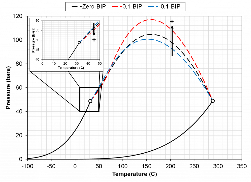
**Figure 3** – Example of how positive (**red** dashed line) and negative (**blue** dashed line) BIPs affects the critical locus of a binary system (C₂-benzene) compared to a zero BIP case (**black** dashed line). The arrows indicate the shift due to an increasing value of the BIP.

From the results of Figure 3, a general trend can be shown. The effect is (a) temperature dependent, (b) dependent on the sign of the BIP and (c) dependent on the magnitude of the BIP. In the temperature region near the light component critical temperature a positive BIP will reduce the critical pressure while a negative BIP will increase the critical pressure. For higher temperatures near the heavy component critical temperature, a positive BIP will increase the critical pressure while a negative BIP will decrease the critical pressure. Another trend that is not shown here is that the magnitude of the critical pressure shift is dependent on the distance between the two component critical temperatures. For a larger difference in component critical temperatures, the larger the difference in the magnitude of the critical pressure.

As indicated in the previous section, the critical pressure locus is directly connected to the high-pressure K-values (i.e. through the convergence pressure), so the shift in the critical pressure will effect the K-value vs pressure plot as well. By picking two temperatures from the two regions with different behavior in the critical pressure shift, gives an indication of the general trend in the K-value behavior with respect to a change in the BIP. Using the same binary system as in the previous examples, a temperature of 50^oC and 175^oC were chosen to show the effect of BIPs on the K-values.

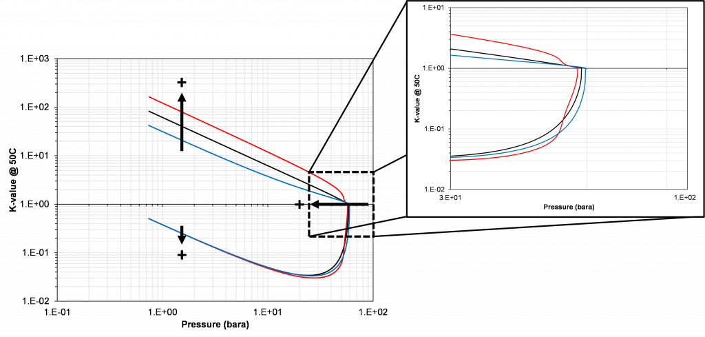
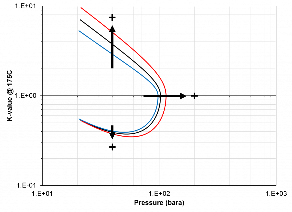
**Figure 4** – Example of how a positive BIP (**red** line) and negative BIP (**blue** line) effect the K-values at 50^oC compared to a zero BIP case (**black** line) for a binary system (C₂-benzene). The arrows on the left plot indicate the how the K-values change when increasing the BIP (toward the + symbol). The right plot is a zoomed plot near the high-pressure region (i.e. near the convergence pressure).

**Figure 5** – Example of how a positive BIP (**red** line) and negative BIP (**blue** line) effect the K-values at 175^oC compared to a zero BIP case (**black** line) for a binary system (C₂-benzene). The plot indicates how the K-values change when increasing the BIP (toward the + symbol).

From Figure 4 and 5 it is apparent that if there is available K-value data, that there is a particular choice of BIP (zero or non-zero) for the binary system that will match the K-value data. Using the results shown in Figure, 3 it is possible to assert how the BIP should be changed to fit the K-value data, i.e. whether the BIP should be increased or decreased. This choice of VLE data is what will be used in this study because of the clear relationship between the value of the BIP and the phase behavior discussed above.

Determining the Values of BIPs

How to determine the values of BIPs can be divided into three procedures, namely (1) taking a set of BIPs from a table, (2) using a correlation in a predictive manner, or (3) tuning the BIPs to available PVT data. All three methods will be discussed in the following section.

The first approach to determine the BIPs of a multi-component system is to take a set of values from a pre-defined table. There are multiple methods that can be used here, but the most common are (a) to use all zero BIPs [6-10], or (b) use non-zero BIPs for NHC isomers and zero BIPs for HC-HC pairs [11,12].

If you choose to only use zero-valued BIPs, Michelsen showed that you can performed a simplified flash, which allows you to explicitly determine the K-values of a mixture as an equation. However, this method is not commonly used, as it has been shown that such a simplification does not accurately predict most real petroleum systems [13,14]. The more common approach is to use zero valued BIPs for HC-HC pairs, while using some pre-determines list of BIPs for NHC components. One justification that has been given for using zero values BIPs is the fact that HC-HC pairs are said to be non-polar [15-19]. This justification will be tested in the next section where HC-HC binary system K-value data will indicate if this claim holds. Another justification for using zero valued BIPs for HC-HC pairs is to avoid non-physical liquid-liquid behavior [20, 21]. This secondary claim will not be investigated in detail in this article but is of upmost importance. A proposed solution to this potential issue is given in the conclusion of this study.

The second method of attaining BIPs, typically for HC-HC pairs, is by using a correlation in a predictive manner. There are a range of different BIP correlations [4, 22-28, 44], but there is in particular one that claims to be predictive and this is a group contribution method (GCM) first proposed by Jaubert et al. [26]. This GCM correlation is based on a semi-analytical model that has been tuned to binary VLE data for many binaries (thousands of data) [29-35]. This method will also be tested using binary K-value data in the next section.

The third approach to attaining BIPs is by tuning them to PVT data. This approach is divided into three main strategies, namely (a) tuning only the lightest component and the heaviest component as proposed by Katz and Firoozabadi [36], (b) by tuning correlation parameters or (c) by tuning the BIPs based on their effect on enhancing the prediction of the PVT data.

The first approach of only tuning the lightest and heaviest HC-HC pair was shown to be a required minimum to fit the phase behavior of certain petroleum fluids in a paper by Katz and Firoozabadi in 1978 [36]. An important finding in this paper was that they were not able to fit the K-value data of their fluid without tuning at least the BIP between the lightest and heaviest HC-HC pair. The second method of attaining BIPs by tuning the correlation parameters to VLE data is a widely used approach and has shown good results for various fluid systems [4, 25]. A hybrid between methods (a) and (b) can also be applied where only a subset of the components is tuned using a correlation. A common correlation used for this approach is the Chueh-Prausnitz correlation as described by Younus et al. [37].

The third approach of using the effect of changing the BIPs on the prediction of the PVT data was proposed by Gani and Fredenslund [38] in 1987, then independently by Liu in 1999 [39] and expanded on by Nielsen in 2020. This approach uses some metric of change in the prediction of PVT data by changing individual BIPs to estimate the effect of changing each BIP. This metric of change is then used to pick a subset of BIP to tune based on the prediction of the PVT data. Nielsen shows that there are some potential issues with these methods if combinations of positive and negative BIPs are introduced, leading to non-physical EOS models (crossing K-values). Nielsen also shows that the BIP between the lightest and heaviest HC-HC pair tends to have the greatest impact on the prediction of the PVT data, validating the work by Katz and Firezoobadi. The reason that only a subset of BIPs is chosen to perform tuning on is the vast number of possible BIPs to tune for real petroleum systems (>1000 BIPs for a detailed EOS model).

Determining the BIP of a Binary Using K-value Data

The results in this section will be divided into two parts, where (1) a comparison between SRK zero BIP model and PR zero BIP model will be conducted for a HC-HC pair, and (2) measured K-value data for known HC pairs will be used to determine (if possible) what the BIP for that specific pair should be to accurately predict the data.

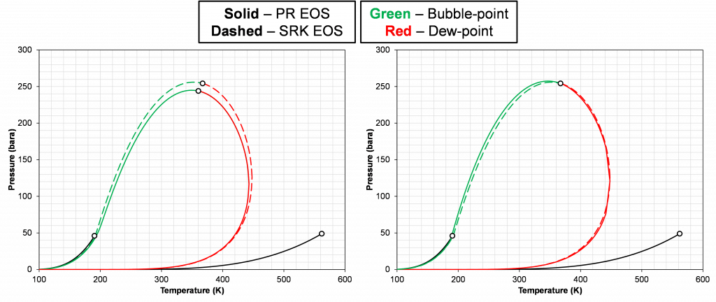
**Figure 6** – Example of mismatch between zero-BIP SRK (dashed lines) and zero-BIP PR (solid lines) EOS models for a C₁-benzene binary system with composition [0.75, 0.25] (left plot). The right plot is the initial composition for the SRK and the critical composition (z_ci such that p_c(z_ci, T_c,SRK)) of the tuned PR EOS with a BIP of 0.02 based on constraint that p_c,PR(T_c,SRK)=p_c,SRK(T_c,SRK). The vapor pressure of C₁ (left) and benzene (right) are also given by a solid black line with the critical points being shown as circles with black marker edges.

The left plot in Figure 6 shows the discrepancy in the phase envelope for a single binary for a given composition. This highlights the fact that the PR and SRK EOS models do not predict the same phase behavior. There is, in fact, various VLE data that can be used to tune the PR EOS model to match the SRK EOS phase behavior. A list of different options is given below:

Critical pressure – p_c,PR(T) = p_c,SRK(T)
Saturation pressure (upper or lower) – p_sat,PR(T) = p_sat,SRK(T)
1. Can also use K-values at saturation pressure – K_i,PR(p_sat,T) = K_i,SRK(p_sat,T)
N datapoints from the equilibrium K-value data – K_i,PR(z_i,p,T) = K_i,SRK(z_i,p,T)
N datapoints of equilibrium compositional data (same as 3) – u_i,PR(z_i,p,T) = u_i,SRK(z_i,p,T)

Even though using method (1) for tuning the PR EOS model, will ensure the same critical pressure, other VLE data will still differ. The right plot in Figure 6 shows an example of this where the critical point is the same for both models, but the phase envelopes are different, and the critical compositions are different (z_i,SRK≠z_ci,PR | [0.75,0.25] vs [0.734,0.266]).

Using the critical point as the only constraint on the model tuning, a temperature BIP relationship can be found. An example of this is shown in Figure 7.

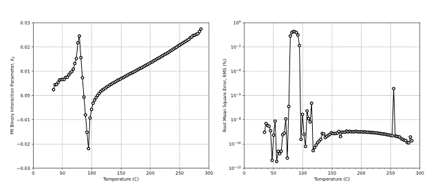
**Figure 7** – Relationship between PR BIP versus temperature (left) and the RMS of the predicted convergence pressure (right) with respect to the SRK zero BIP EOS model for a C₂-benzene binary system.

There are several interesting points to note about the results in Figure 7. First, the BIP relating the tuned PR EOS with the zero BIP SRK EOS model is not zero. Second, there seems to be a discontinuity in the value of the BIP at approximately 90^oC where the predicted BIP results in a higher RMS value. Finally, a negative BIP is predicted to give the best result for modeling the zero BIP SRK EOS model. This indicates that to recreate a certain segment of the zero BIP SRK model you need to have a negative BIP. This sheds some light on the fact that negative BIPs should not be thought of as “non-physical”. However, Nielsen showed that a combination of positive and negative BIPs can result in non-physical low-pressure K-value crossing.

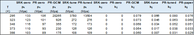
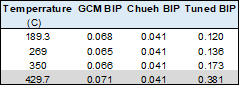
In the following figures, various hydrocarbon-hydrocarbon pairs are shown using measured K-value data and different BIP estimates. The different binary pairs are:

Ethane and benzene (single temperature)
Methane and 1-methylnaphthalene (5 temperatures)
Methane and 1-diphenalmethane (4 temperatures)
Methane and normal decane (5 temperatures)

The different BIP estimates used are:

Zero BIP PR
Zero BIP SRK
Tuned BIP PR
Tuned BIP SRK
GCM BIP PR

**Figure 8** – Example of binary K-value data (**black** x symbol) for C₂-benzene mixture at 25^oC. The different models are (a) zero BIP PR (**blue** line), (b) zero BIP SRK (**green** line), (c) GCM BIP with PR EOS (**pink** line), and (d) tuned BIP with PR EOS (**red** line). The tuned BIP was tuned to the C₂ data [40].

**Figure 9** – K-value data for binary mixture containing C₁ and 1-methylnaphthalene [41] at temperatures ranging from 295K (top left), 323K (top right), 348K (middle left), 373K (middle right), and 398K (bottom). The different models are (a) zero BIP PR (**blue** circle marker), (b) zero BIP SRK (**red** circle marker), (c) GCM BIP with PR EOS (**pink** square maker), and (d) tuned BIP with PR EOS (**black** diamond marker). The tuned BIP was tuned to the C₂ data.

**Figure 10** – K-value data for binary mixture of C1 and 1-diphenalmethane [42] at temperatures ranging from 189.3C (top left), 269C (top right), 350C (bottom left) and 429.7C (bottom right) indicated by a black line with black circular markers. The model predictions are indicated by color, where **red** is the GCM correlation using the PR EOS, **green** is the Chueh-Prausnitz correlation with the PR EOS, and **pink** is the zero BIP PR EOS.

**Figure 11** – K-value data for binary mixture of C₁ and n-C₁₀ [43] at temperatures ranging from 150C (top left), 237.8C (top right), 269.6C (middle left), 290.1C (middle right), 309.9C (bottom left) indicated by circular markers. The model predictions are indicated by color (**red** is PR and **black** is SRK), line type (solid is zero BIP, long dash is tuned by method 1, short dash is tuned by method 2), and the **pink** line is using the predictive GCM correlation.

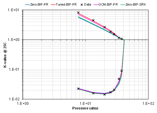
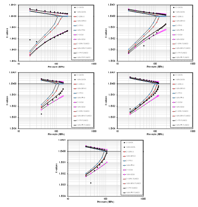
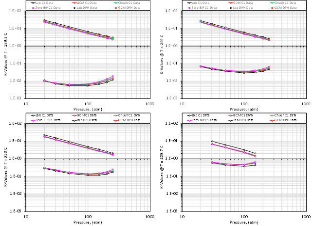
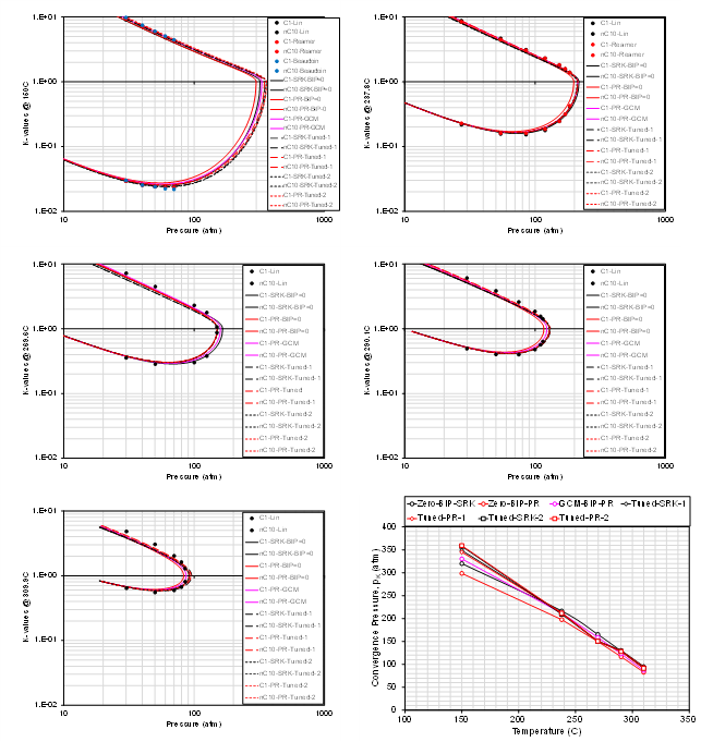
These are only a small subset of binary systems, but the trend shows that there is (a) a clear deviation from zero BIP EOS models (PR and SRK) for specific binaries at certain temperatures, and (b) that there is a significant spread in the prediction of K-values based on the different models. This trend holds for various hydrocarbon types (paraffins, aromats and naphthenes). The data also shows that the predictive ability of the GCM correlation varies with respect to the binary pair in question.

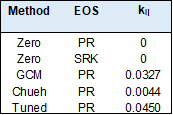
Some of the results from the models used are given in the tables below.

**Table 1** – Results from K-value data given in Figure 8.

**Table 2** – Results from convergence pressure for mixture shown in Figure 9.

**Table 3** – Results from convergence pressure for mixture shown in Figure 10. The data from the last dataset is greyed out because there is significant uncertainty in the data.

Conclusions

There is a significant difference between the PR and SRK EOS models when using zero valued BIPs, so it is not consistent to state that zero BIPs should be used for both EOS models, if any at all. This is a fact for ANY components whether they are polar or non-polar, HC-HC or NHC-HC.
Both negative and positive BIPs are needed to reproduce a zero BIP SRK EOS model with a tuned PR EOS model.
The results of fitting one EOS model to another using only the BIP will (a) depend on the VLE data used to fit the model, and (b) will not predict all VLE data to an arbitrary degree of accuracy.
For HC-HC binary pairs, the BIP needed to predict the measured K-value is (a) seldom equal to zero and (b) is always temperature dependent.
Zero BIPs is a default choice and needs to be justified just like the choice of any other unknown correction term.
Even though non-zero BIPs are often needed and used, it is important to state that non-physical behavior can occur and needs to be checked using QCs like K-value crossing and three phase checks [20, 21,37]. A specific example of this behavior is for a C₁-benzene binary at temperatures near the critical temperature of C₁.
More research needs to be published on the constraints of BIP tuning that ensures physical consistency. Currently there are only rule-of-thumb approaches like (a) the BIPs should be monotonically increasing, or (b) the BIPs should vary “smoothly”.

Learn more about our consulting capabilities

###

Global
Curtis Hays Whitson
curtishays@whitson.com

Asia-Pacific
Kameshwar Singh
singh@whitson.com

Middle East
Ahmad Alavian
alavian@whitson.com

Americas
Mathias Lia Carlsen
carlsen@whitson.com

About whitson
whitson supports energy companies, oil services companies, investors and government organizations with expertise and expansive analysis within PVT, gas condensate reservoirs and gas-based EOR. Our coverage ranges from R&D based industry studies to detailed due diligence, transaction or court case projects. We help our clients find the best possible answers to complex questions and assist them in the successful decision-making on technical challenges. We do this through a continuous, transparent dialog with our clients – before, during and after our engagement. The company was founded by Dr. Curtis Hays Whitson in 1988 and is a Norwegian corporation located in Trondheim, Norway, with local presence in USA, Middle East, India and Indonesia

References

[1] Van der Waals, J., 1873. On the continuity of the gaseous and liquid states (doctoral dissertation). Universiteit Leiden.

[2] Peng, D.Y., Robinson, D.B., 1978. The characterization of the heptanes and heavier fractions for the GPA Peng-Robinson programs. Gas processors association.

[3] Soave, G., 1972. Equilibrium constants from a modified Redlich-Kwong equation of state. Chemical engineering science 27, 1197–1203.

[4] Chueh, P., Prausnitz, J., 1967. Vapor-liquid equilibria at high pressures: Calculation of partial molar volumes in nonpolar liquid mixtures. AIChE journal 13, 1099–1107.

[5] Gibbs, J.W., 1961. The Scientific Papers, Vol I: Thermodynamics. Dover Publications. (Gibbs phase rule)

[6] Michelsen, M.L., 1986. Simplified flash calculations for cubic equations of state. Industrial & Engineering Chemistry Process Design and Development 25, 184–188.

[7] Jensen, B.H., Fredenslund, A., 1987. A simplified flash procedure for multicomponent mixtures containing hydrocarbons and one non-hydrocarbon using two-parameter cubic equations of state. Industrial & engineering chemistry research 26, 2129–2134.

[8] Hendriks, E.M., 1988. Reduction theorem for phase equilibrium problems. Industrial & engineering chemistry research 27, 1728–1732.

[9] Hendriks, E.M., 1988. Reduction theorem for phase equilibrium problems. Industrial & engineering chemistry research 27, 1728–1732.

[10] Hendriks, E., Van Bergen, A., 1992. Application of a reduction method to phase equilibria calculations. Fluid Phase Equilibria 74, 17–34.

[11] Reid, R.C., Prausnitz, J.M. and Sherwood, T.K., 1977. The Properties of Liquids and Gases.(Stichworte Teil 2). McGraw-Hill.

[12] Knapp, H., Doring, R., Oellrich, L., Plocker, U. and Prausnitz, J.M., 1982. Vapor-liquid equilibria for mixtures of low-boiling substances, Dechema Chemistry Data Series, Vol. VI, Frankfurt/Main.

[13] Haugen, K.B., Beckner, B.L., et al., 2011. Are reduced methods for eos calculations worth the effort?, in: SPE Reservoir Simulation Symposium, Society of Petroleum Engineers.

[14] Michelsen, M., Yan, W., Stenby, E.H., et al., 2013. A comparative study of reducedvariables- based flash and conventional flash. SPE Journal 18, 952–959.

[15] Pedersen, K.S., Thomassen, P. and Fredenslund, A., 1984. Thermodynamics of petroleum mixtures containing heavy hydrocarbons. 1. Phase envelope calculations by use of the Soave-Redlich-Kwong equation of state. Industrial & Engineering Chemistry Process Design and Development, 23(1), pp.163-170.

[16] Pedersen, K.S., Thomassen, P. and Fredenslund, A., 1988. On the dangers of “tuning” equation of state parameters. Chemical engineering science, 43(2), pp.269-278.

[17] Pedersen, K.S., Thomassen, P. and Fredenslund, A., 1988. Characterization of gas condensate mixtures (No. CONF-880348-). New York, NY; American Institute of Chemical Engineers.

[18] Aasberg-Petersen, K. and Stenby, E., 1991. Prediction of thermodynamic properties of oil and gas condensate mixtures. Industrial & engineering chemistry research, 30(1), pp.248-254.

[19] Aoki, T., Furuta, T., Leekumjorn, S., Azeem Shaikh, J., Schou Pedersen, K., Alobeidli, A. and Mogensen, K., 2020, November. A New Technique for Common EoS Model Development for Multiple Reservoir Fluids with Gas Injection. In Abu Dhabi International Petroleum Exhibition & Conference. Society of Petroleum Engineers.

[20] Pedersen, K.S., Milter, J. and Sørensen, H., 2002, January. Cubic equations of state applied to HT/HP and highly aromatic fluids. In SPE Annual Technical Conference and Exhibition. Society of Petroleum Engineers.

[21] Krejbjerg, K. and Pedersen, K.S., 2006, January. Controlling VLLE equilibrium with a cubic EOS in heavy oil modeling. In Canadian International Petroleum Conference. Petroleum Society of Canada.

[22] Mathias, P.M., 1983. A versatile phase equilibrium equation of state. Industrial & Engineering Chemistry Process Design and Development, 22(3), pp.385-391.

[23] Nishiumi, H., Arai, T. and Takeuchi, K., 1988. Generalization of the binary interaction parameter of the Peng-Robinson equation of state by component family. Fluid Phase Equilibria, 42, pp.43-62.

[24] Slot-Petersen, C., 1989. A systematic and consistent approach to determine binary interaction coefficients for the Peng-Robinson Equation of State (includes associated papers 20308 and 20393). SPE reservoir engineering, 4(04), pp.488-494.

[25] Coutinho, J.A., Kontogeorgis, G.M. and Stenby, E.H., 1994. Binary interaction parameters for nonpolar systems with cubic equations of state: a theoretical approach 1. CO2/hydrocarbons using SRK equation of state. Fluid phase equilibria, 102(1), pp.31-60.

[26] Jaubert, J.N., Mutelet, F., 2004. Vle predictions with the peng–robinson equation of state and temperature dependent kij calculated through a group contribution method. Fluid Phase Equilibria 224, 285–304.

[27] Fateen, S.E.K., Khalil, M.M. and Elnabawy, A.O., 2013. Semi-empirical correlation for binary interaction parameters of the Peng–Robinson equation of state with the van der Waals mixing rules for the prediction of high-pressure vapor–liquid equilibrium. Journal of advanced research, 4(2), pp.137-145.

[28] Abudour, A.M., Mohammad, S.A., Robinson Jr, R.L., Gasem, K.A., 2017. Predicting pr eos binary interaction parameter using readily available molecular properties. Fluid Phase Equilibria 434, 130–140.

[29] Jaubert, J.N., Vitu, S., Mutelet, F., Corriou, J.P., 2005. Extension of the ppr78 model (predictive 1978, peng–robinson eos with temperature dependent kij calculated through a group contribution method) to systems containing aromatic compounds. Fluid Phase Equilibria 237, 193–211.

[30] Vitu, S., Jaubert, J.N., Mutelet, F., 2006. Extension of the ppr78 model (predictive

1978, peng–robinson eos with temperature dependent kij calculated through a group contribution method) to systems containing naphtenic compounds. Fluid phase equilibria 243, 9–28.

[31] Vitu, S., Privat, R., Jaubert, J.N., Mutelet, F., 2008. Predicting the phase equilibria of co2+ hydrocarbon systems with the ppr78 model (pr eos and kij calculated through a group contribution method). The Journal of Supercritical Fluids 45, 1–26.

[32] Privat, R., Jaubert, J.N., Mutelet, F., 2008a. Addition of the nitrogen group to the ppr78 model (predictive 1978, Peng Robinson EOS with temperature-dependent kij calculated through a group contribution method). Industrial & engineering chemistry research 47, 2033–2048.

[33] Privat, R., Jaubert, J.N., Mutelet, F., 2008b. Use of the ppr78 model to predict new equilibrium data of binary systems involving hydrocarbons and nitrogen. comparison with other gceos. Industrial & engineering chemistry research 47, 7483–7489.

[34] Jaubert, J.N., Privat, R., 2010. Relationship between the binary interaction parameters (kij) of the peng–robinson and those of the soave–redlich–kwong equations of state: Application to the definition of the pr2srk model. Fluid Phase Equilibria 295, 26–37.

[35] Jaubert, J.N., Privat, R., Mutelet, F., 2010. Predicting the phase equilibria of synthetic petroleum fluids with the ppr78 approach. AIChE journal 56, 3225–3235.

[36] Katz, D., Firoozabadi, A., et al., 1978. Predicting phase behavior of condensate/crude-oil systems using methane interaction coefficients. Journal of Petroleum Technology 30, 1–649.

[37] Younus*, B., Whitson, C.H., Alavian, A., Carlsen, M.L., Martinsen, S.Ø., Singh, K., 2019. Field-wide equation of state model development, in: Unconventional Resources Technology Conference, Denver, Colorado, 22-24 July 2019, Unconventional Resources Technology Conference (URTeC); Society of . . . . pp. 1031–1070.

[38] Gani, R. and Fredenslund, A., 1987. Thermodynamics of petroleum mixtures containing heavy hydrocarbons: an expert tuning system. Industrial & engineering chemistry research, 26(7), pp.1304-1312.

[39] Liu, K., 1999, January. Fully automatic procedure for efficient reservoir fluid characterization. In SPE Annual Technical Conference and Exhibition. Society of Petroleum Engineers.

[40] Ohgaki, K., Sano, F. and Katayama, T., 1976. Isothermal vapor-liquid equilibrium data for binary systems containing ethane at high pressures. Journal of Chemical and Engineering Data, 21(1), pp.55-58.

[41] Marteau, P., Tobaly, P., Ruffier-Meray, V. and Barreau, A., 1996. In situ determination of high pressure phase diagrams of methane-heavy hydrocarbon mixtures using an infrared absorption method. Fluid phase equilibria, 119(1-2), pp.213-230.

[42] Sebastian, H.M., Simnick, J.J., Lin, H.M. and Chao, K.C., 1979. Gas-liquid equilibrium in binary mixtures of methane with tetralin, diphenylmethane, and 1-methylnaphthalene. Journal of Chemical and Engineering Data, 24(2), pp.149-152.

[43] Lin, H.M., Sebastian, H.M., Simnick, J.J. and Chao, K.C., 1979. Gas-liquid equilibrium in binary mixtures of methane with n-decane, benzene, and toluene. Journal of Chemical and Engineering Data, 24(2), pp.146-149.

[44] Gao G, Daridon JL, Saint-Guirons H, Xans P, Montel F. A simple correlation to evaluate binary interaction parameters of the Peng-Robinson equation of state: binary light hydrocarbon systems. Fluid phase equilibria. 1992 Jul 15;74:85-93.