By Bilal Younus, July 2021
This article discusses two common molar distribution models – discrete exponential and continuous gamma – used to describe heavier components such as heptanes-plus (C7+) in petroleum reservoir fluids.
A molar distribution model relates component molar amount (mole fraction) to molecular weight (MW). The discrete exponential distribution is used exclusively to relate single-carbon-number (SCN) mole fraction to SCN molecular weight. The continuous gamma distribution model can describe SCN fractions, but it also can be used to describe true boiling point data where each distillation cut contains a range of SCN compounds defined by the cut’s boiling-point range.
Gas chromatography (GC) is the most common technique for measuring compositions of the heavier C7+ components in a petroleum mixture. Mass amounts of SCNs and a heavy residue (CN+) are measured on atmospheric oil samples. In the past decade it has become standard that GC reports the mass quantity of important isomers (e.g. BTEX) in the C6–C9 range.
We recommend using lab-reported GC mass amounts to fit the molar distribution model. Mass amounts from the molar distribution model are readily calculated from fraction molar amounts and model MWs of the fractions.
Approximate molar composition of C7+ components is calculated by the lab from measured GC mass fractions and a set of assumed component molecular weights, usually from Katz and Firoozabadi (1978). We seldom use the lab-reported molar compositions. Instead, molar amounts are calculated using lab-reported mass amounts and the EOS molecular weights (usually from the molar distribution model).
The continuous gamma distribution model can better describe measured SCN distributions because each SCN MW range varies (14±6). This is an important characteristic when building multi-sample, field-/basin-wide EOS models, where we find that that the MW range varies for each SCN, but that the SCN MW ranges are the same for all samples. The discrete exponential model has a fixed MW range of 14 for all SCNs.
In the treatment below, we use normalized mole fractions \(\hat{z}\) in a Cn+ distribution model, with the final residue (heaviest fraction) being expressed as CN+.
Discrete Exponential Model
The discrete exponential model as given by Whitson and Brule (2000) is
| $$ẑ_i=ẑ_n exp[A(i-n)]$$ | (1) |
where n is the first heavy SCN in the distribution and i = n, n+1, … N-1, with
| \(\hat{z}_i = z_i/z_{n+}\) and \(\hat{z}_n = z_n/z_{n+}\) | (2) |
| \(\hat{z}_n = \frac{14}{M_{n+}-14(n-1)-h}\) and \(A = ln(1-z_n)\) | (3) |
\(\hat{z}_n\) is the normalized mole fraction of carbon number i. The term h is related to the number of hydrogen atoms per carbon atom, and is assumed to be a constant value (e.g. h=-4 in PVTSim). SCN average MWs are given by
| $$M_i = 14i + h$$ | (4) |
The discrete exponential model plots as a linear relation for log(\(\hat{z}_i\)) vs Mi, with slope A and intercept \(\hat{z}_n\), both controlled by the average molecular weight Mn+. Another assumption in the model is that all component MWs are equally spaced, Mi+1 – Mi = 14, because h is constant. Normalized mass fraction \(\hat{w}_i\) in the Cn+ mixture is given by
| $$\hat{w}_i = \hat{z}_i M_i / M_{n+}$$ | (5) |
Note that log(\(\hat{w}_i\)) vs Mi from the exponential model is not linear, and may result in a non-monotonic mass fraction trend.
Gamma Distribution Model
The continuous gamma distribution model (Whitson 1980,1983) is based on the three-parameter gamma probability density function:
| $$p(M)=\frac{(M-η)^{α-1}exp[-(M-η)/β])}{β^α Γ(α)}$$ | (6) |
with the three parameters α and β, with β = (Mn+-η)/α. The parameter α controls the shape of the distribution, and η is the lowest molecular weight in the distribution (Fig. 1). Most reservoir fluids have a gamma shape best fit parameter ranging from 0.5 to 1.5, with α=1 representing a continuous exponential distribution. Biodegraded reservoir fluids tend to show α>1.5. Oil based muds, heavy oils and oil residues can have α ranging from 5 to 20. α=∞ yields a folded log-normal distribution.
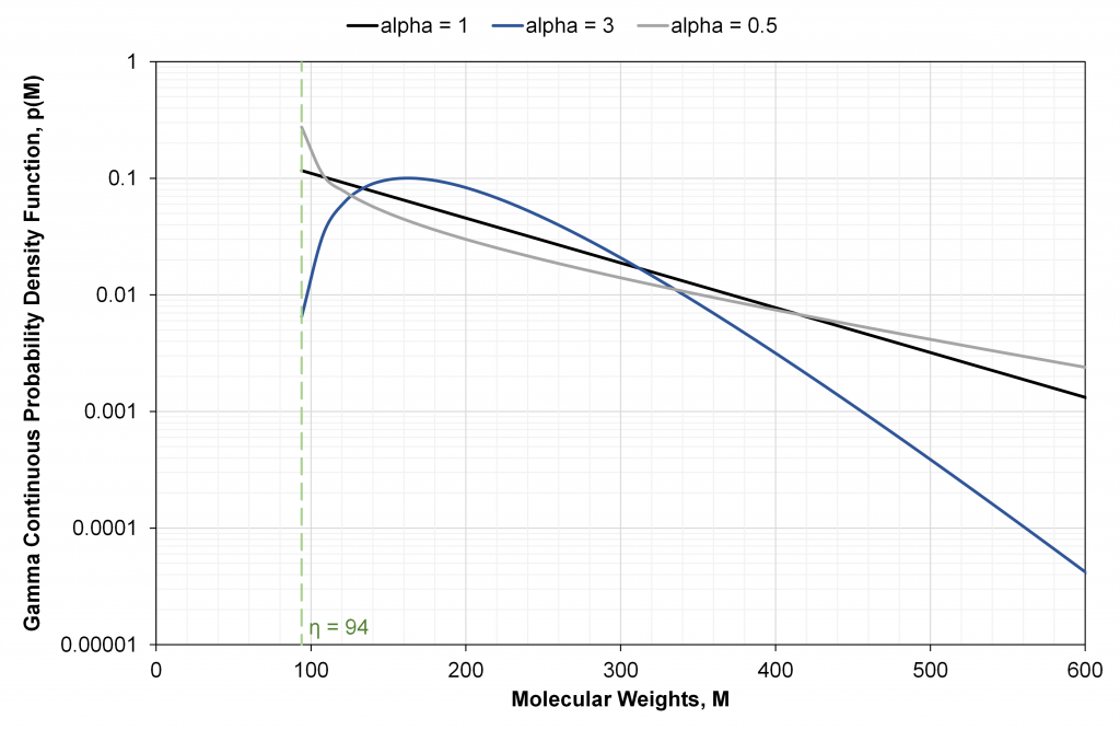
The η value is always less than the MW of the first Cn+ fraction Mn. For example, C7+ has a first SCN C7 that contains isomers from benzene (M=78) to n-C7 (M=100), so we expect 78<η<100.
The average Cn+ molecular weight Mn+ is known with reasonable certainty (±2-10%) from laboratory measurement.
Integrating the probability density function p(M) from M=η to ∞ yields 1, the total Cn+ normalized mole fraction. Integrating M p(M) from M=η to ∞ yields the total Cn+ average MW (Mn+).
An arbitrary “cut” k between any two “lower” MW bounds (ML,k and ML,k+1) will yield the cut’s normalized mole fraction \(\hat{z}_k\) and average molecular weight Mk, calculated by appropriate integration of the gamma distribution model.
For illustration purpose only, Fig. 1 uses a small and constant MW bounding interval to yield a relation of mole fraction to molecular weight that mimics the shape of the actual probability density function p(M). If instead we selected variable MW bounding intervals for each cut, then the resulting shape of individual cut mole fraction versus individual cut MW could be made to increase, exhibit non-monotonic behavior, or remain constant (i.e. each cut with an equal mole fraction).
Judicious selection of individual cut (e.g. SCN) bounding MWs (ML,k) is an important feature of the continuous gamma distribution model, and its success in providing a consistent description for a wide range of petroleum mixtures that are experimentally quantified with a variety of laboratory methods (gas chromatography and distillation).
The discrete exponential distribution can be calculated exactly from the continuous gamma model using when α = 1, lower MWs MLi = (14i + h) – 7, and η = MLn = (14n + h) – 7 (n=first carbon number in the distribution).
As mentioned earlier, the normalized mass fraction between two bounds of a cut is given by Equation 5. We always recommend converting molar amounts from the gamma distribution model to mass fractions – to compare with and fit laboratory measured mass fractions (instead of using approximate lab-reported mole fractions based on assumed molecular weights).
Exponential and Gamma Models Applied to Petroleum Systems
With extended GC data available on most samples in a field or basin, we try to develop a common gamma molar distribution model for C7+ (or C10+) that is applicable to all samples. The field-wide gamma model generally has a common shape (α), lower MW bounds (MLi), where η = MLn , and sample-specific average MWs (Mn+).
Most samples show an excellent match between the laboratory SCN mass fractions and the gamma model SCN mass fractions (Younus et al, 2019). Some samples show a good match up to some carbon number (e.g. C20), but significant deviation for heavier SCNs. This behavior is usually linked to GC laboratory procedures involving internal standard and baseline shift issues. The common gamma model provides a quantitative QC of lab data. Utilizing the gamma model to quantify errors in measured mass fractions of Cn+ components is described in detail in our course videos at Whitson Academy (https://academy.whitson.com).
A common gamma model also provides SCN MWs (and MW of the heaviest fraction CN+), consistent with GC data, and often used in our EOS model development.
In the figures below, we have shown four examples of field-wide (tuned) gamma models describing the measured mass fractions of C7+ components (one conventional field and three tight unconventional basins). We also show the discrete exponential with h = -4 and using the same M7+ as used by the gamma model.
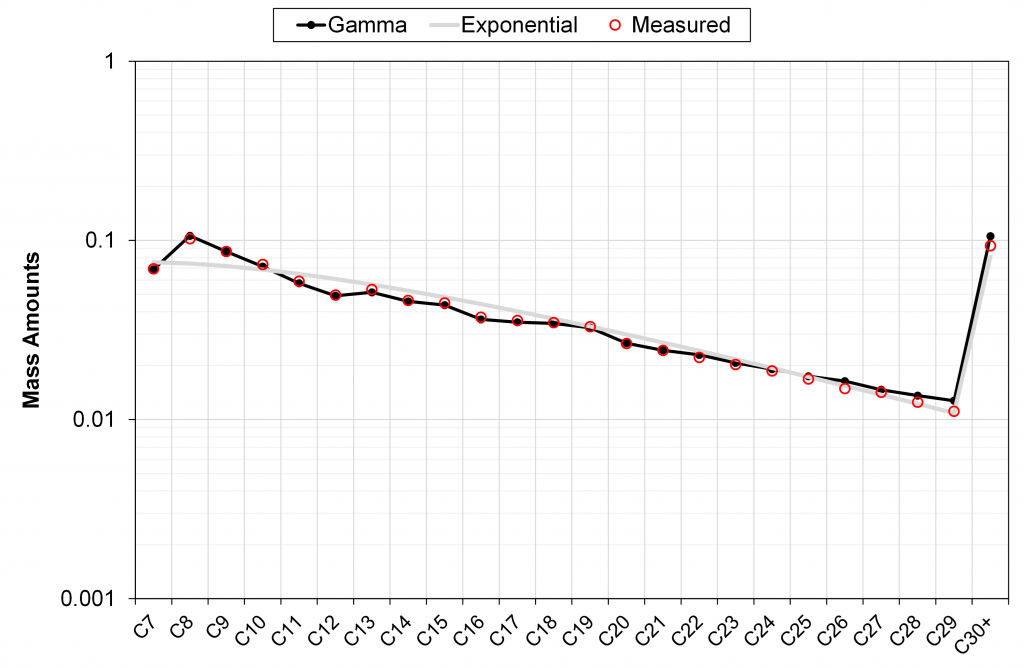
Figure 2 – Comparison of calculated C7+ mass fractions from discrete exponential model and field-wide tuned gamma model versus lab measured data. Field-wide gamma model is tuned to 60+ PVT samples in the same field.
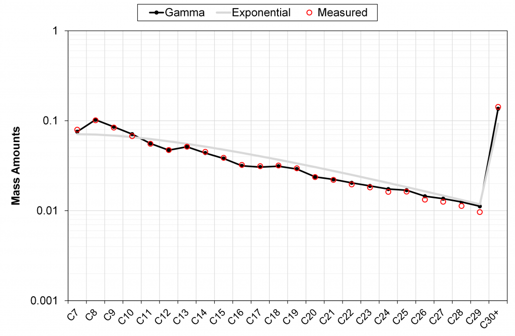
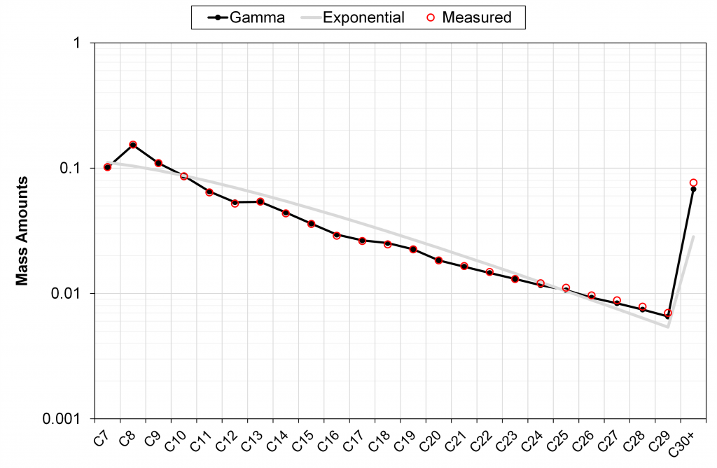
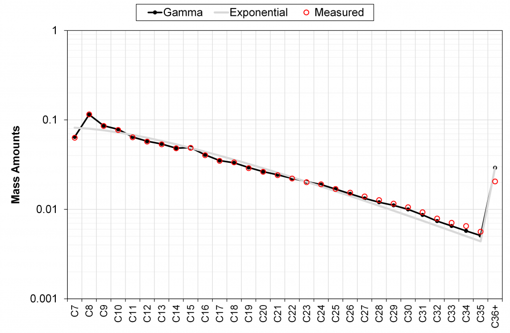
It can be seen in these different examples that the field-wide tuned gamma model accurately describes the measured mass distribution of C7+ fractions, unlike the discrete exponential model with only a single (sample-specific) tuning parameter M7+.
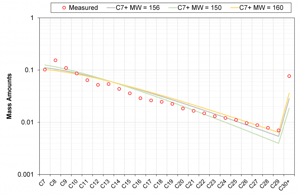
The impact of M7+ on C7+ mass distribution from the discrete exponential model is shown below.
Learn more about our consulting capabilities
###
Global
Curtis Hays Whitson
curtishays@whitson.com
Asia-Pacific
Kameshwar Singh
singh@whitson.com
Middle East
Ahmad Alavian
alavian@whitson.com
Americas
Mathias Lia Carlsen
carlsen@whitson.com
About whitson
whitson supports energy companies, oil services companies, investors and government organizations with expertise and expansive analysis within PVT, gas condensate reservoirs and gas-based EOR. Our coverage ranges from R&D based industry studies to detailed due diligence, transaction or court case projects. We help our clients find the best possible answers to complex questions and assist them in the successful decision-making on technical challenges. We do this through a continuous, transparent dialog with our clients – before, during and after our engagement. The company was founded by Dr. Curtis Hays Whitson in 1988 and is a Norwegian corporation located in Trondheim, Norway, with local presence in USA, Middle East, India and Indonesia
References
Katz, D. L., & Firoozabadi, A. (1978). Predicting Phase Behaviour of Condensate/Crude-Oil Systems Using Methane Interaction Coefficients. doi: 10.2118/6721-PA
Whitson, C. H. (1983). Characterizing Hydrocarbon Plus Fractions. Society of Petroleum Engineers Journal, 23(04). doi: 10.2118/12233-PA | Original presentation (1980) EUR183, SPE12233.
Whitson, C.H. and Brule, M.R. (2000). Phase Behavior, SPE monograph volume 20.
Younus et al. (2019). Field-wide Equation of State Model Development, URTeC 551