Analytical vs. Numerical RTA

Author: Ilina Yusra

Analyzing infinite-acting linear flow using the square root of time plot has been important in tight unconventional reservoirs since it was first introduced in 1988 by Wattenbarger et al. The goal of the analysis is to determine the fundamental reservoir parameters by solving the analytically derived equations for the two flow regimes a fractured well experiences, the infinite-acting (IA) and the boundary-dominated flow (BDF) period. By combining the linear flow parameters (LFP = A√k), derived from the IA period, with the estimated stimulated rock volume (SRV), derived from the BDF period, we can solve for permeability (k) and fracture half-length (x_f). This interpretation requires careful consideration because it will have significant impact on future field development & optimization plans and ultimately on the economic aspect.

In this article, we will discuss the differences between analytical- (ARTA) and numerical RTA (NRTA). This will include highlighting their advantages and limitations, along with demonstrating when they can be used in practice, by looking at an example using field data.

What is Analytical RTA?

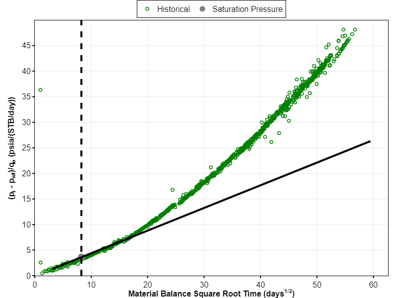
Traditional RTA, or what we refer to as analytical RTA (ARTA), is the most common RTA method in tight unconventional reservoirs. As exemplified in Fig. 1, it involves plotting the rate-normalized pressure (RNP), (p_i-p_wf)/q versus the square root of material balance time, √t based on the following equation

$$\frac{\Delta p}{q}=\frac{p_i-p_{wf}}{q}=m\sqrt{t}+b’$$

(1)

ARTA is a straightforward method in which the infinite-acting linear flow period will exhibit a straight line in the square root of time plot. The slope of the straight line specifies the linear flow parameter (LFP). When one, or more, boundaries are reached, the curve starts to deviate from the straight line, indicating the end of linear flow. The time to end of linear flow (t_elf) is key to specify the drainage volume inside the stimulated rock volume (SRV). With this known LFP and t_elf, we can resolve k and x_f. The complete equations for both reservoir oil and gas can be seen in whitson⁺ manual.

ARTA is a relatively simple method, as it requires only production data (rates and pressures) and initial fluid properties (formation volume factor, viscosity, and compressibility). No special tool is needed to do the analysis. However, the analysis derived on the assumption of single-phase flow, which is rarely the case in tight unconventionals. Furthermore, the method uses PVT properties at initial reservoir pressure and assumes that these values are constant throughout the well’s lifetime. However, as we very well know, the fluid properties change with pressure, especially when two phases are formed at pressure below the saturation pressure (p_sat). Therefore, this assumption is only good for dry and wet gas reservoir, and for wells producing with p_wf above p_sat. But when p_wf drops below p_sat, this method is no longer valid as it will alter the slope of the linear flow in the square root of time plot. In this scenario, it may seem as if the reservoir is seeing boundary effects, while in fact the change of slope is due to multiphase flow effects. Another limitation of this analysis is that the curve in the RNP vs. √t plot is strongly influenced by the complex superposition of solutions due to changing pressures and rates.

What is Numerical RTA?

Bowie and Ewert (2020) presented a new method to enhance the traditional RTA workflow for unconventional oil wells by using a numerical model (reservoir simulation). The proposed analysis solves the problem of multiphase flow effects and complex superposition in ARTA. Carlsen et al. (2021) extended the work by:

• including porosity to modified LFP term,
• introducing the concept of cumulative LFP’s to reduce noise,
• expanding the application of the method for all fluid systems, and
• expanding the method to finite conductivity fractures (low F_cd).

The LFP and estimated drainage volume for an oil reservoir are given by

$$LFP’=LFP\sqrt{\phi}=4n_fx_fh\sqrt{k}\sqrt{\phi}$$

(2)

$$OOIP=\frac{2x_fLh\phi (1-S_{wi})}{B_{ti}}$$

(3)

The new method relies on three fundamental relationships between LFP’, OOIP and well performance:

1. Wells with the same value of LFP’ have the same well performance during IA linear flow.
2. Wells with the same LFP’/OOIP exhibit the same relative rates (producing GOR and water cuts) for all times (IA and BDF).
3. Wells with the same LFP’ and OOIP have the same well performance for all times (IA and BDF).

These relationships apply for wells with the same fluid initialization (PVT and S_wi), relative permeability curves, and flowing bottomhole pressure profile. The workflow starts by creating and running simulation model sufficiently large to remain in the IA period throughout the historical time (for this model we know the LFP’). This model is controlled by the measured (or estimated by correlations) p_wf profile. The LFP’ in every timestep can be calculated by multiplying the daily ratio between the actual measured rates and the IA model rates (r = q_o,actual/q_o,IA or cumulative LFP’ by r = Q_o,actual/Q_o,IA) with the known LFP’ of the IA model. A representative LFP’ can be picked based on horizontal flat line in the early time that indicates the IA linear flow period. The steps are repeated for smaller OOIP to create several type curves of LFP’/OOIP. The curve that best represents the historical data is selected. OOIP is obtained by multiplying LFP’/OOIP with the representative LFP’. The matrix permeability and fracture half-length are calculated by solving Eqs. (2) and (3). For the complete explanation on the workflow please refer to Carlsen et al. (2020) or whitson⁺ manual. A webinar about this method can be seen here.

By utilizing a full-physics numerical model, we can accurately account for time and spatial changes in pressure, composition, PVT properties, and fluid saturations. Additionally, the resulting reservoir property estimates can be exported directly to a higher order analysis (e.g. history matching) without losing the accuracy of the results. However, it is difficult to determine OOIP or minimum drainage volume if the historical well data still only predicts the IA period, consequently making it difficult to calculate the representative k_m and x_f. Like any numerical model, the method depends on the fluid initialization (PVT and S_wi), relative permeability, bottomhole pressure profile, and their respective uncertainties. Changing fluid initialization or relative permeabilities is the recommended first step such that the simulated IA model gives: (1) producing GORs that are equal to or less than the historical, and (2) similar water-cut profile to the historical in the late time (simulation models tend to poorly predict early-time flowback of water). It is worth to mention that this method is still in the early stages which allows further development in the future, e.g. to account for reservoir heterogeneities such as uneven frac spacing.

Case Study

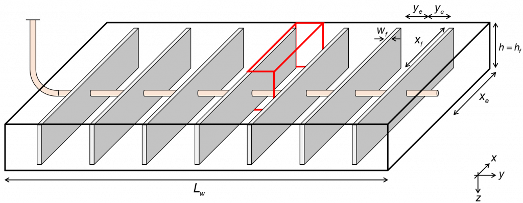
Both ARTA and NRTA methods assume a wellbox model as depicted in Fig. 3, with no flow beyond the tip of the fracture (x_e = x and h = h_f). This section illustrates the differences between ARTA and NRTA through an example with field data. The exercises are carried out using whitson⁺ software.

The data used for this example is Well 4 from dataset 1 of SPE Data Repository. The initial pressure is 6,600 psia, reservoir temperature is 237 °F and initial GOR is 750 scf/STB. The well is producing with flowing bottomhole pressure as shown in Fig. 4, in which the pressure drops below the predicted p_sat after 120 days.

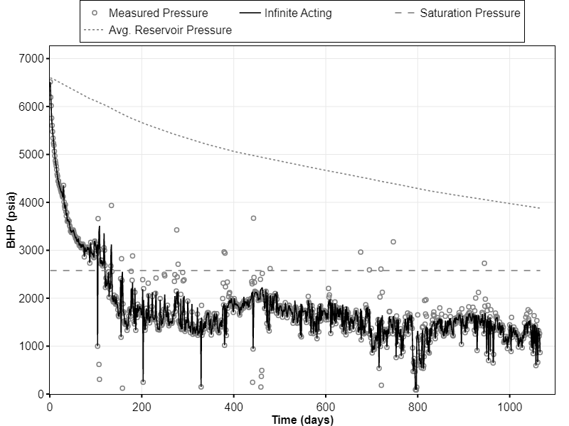
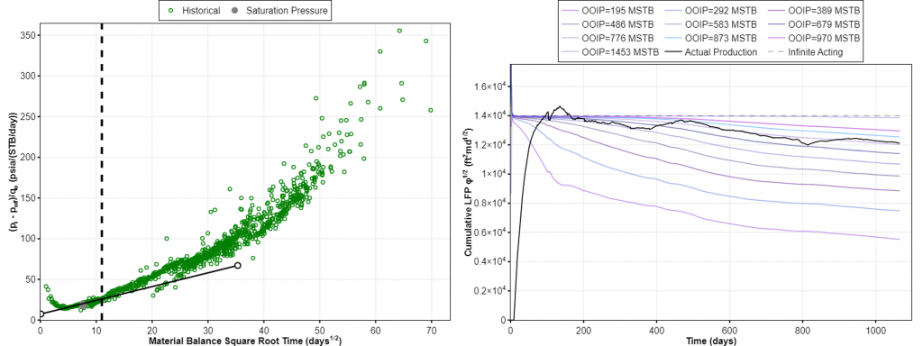
Fig. 5 shows ARTA and NRTA plot for this well. The straight line on the square root of time plot (left plot) suggests an intercept larger than zero, indicating a near-wellbore pressure drop by e.g. skin and/or finite fracture conductivity. The selected straight line also suggests that IA linear flow ends when p_wf drops below p_sat. This interpretation results in OOIP = 454 MSTB and LFP = 49,233 ft²md^1/2, which in turn gives k_m = 12.7 nd and x_f = 199.5 ft.

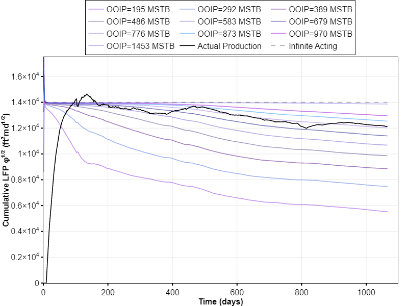
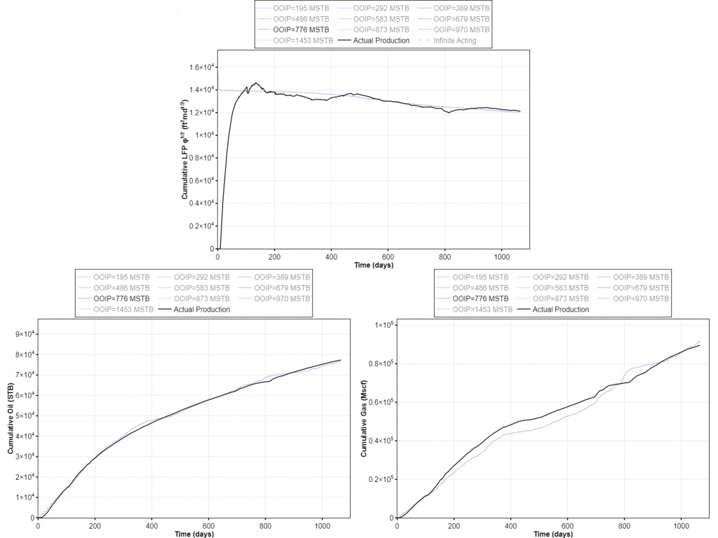
Looking at the cumulative LFP’ plot in Fig. 5 (right plot), the actual production crosses several type curves, but is approximately equal to the stem of OOIP = 776 MSTB as seen in Fig. 6. This number is 1.7x higher than what is estimated by ARTA. Calculating LFP from LFP’ yields LFP = 62,610 ft²md^1/2. This results in k_m = 8.6 nd and x_f = 311.2 ft.

The complete comparison of the results is summarized in table below. The values of LFP and OOIP from ARTA can be misleading and will in most cases yield a smaller in-place estimate than reality. Smaller OOIP leads to shorter x_f and higher k_m, which would suggest tighter well spacing than optimal (i.e. overcapitalization). This field example shows that it is relevant and necessary to verify the ARTA results with NRTA, especially when the well is producing at flowing bottomhole pressure below the saturation pressure.

Parameter	Units	Analytical RTA	Numerical RTA
nf	#	306	306
L	ft	5,086	5,086
Frac spacing	ft	16.6	16.6
h	ft	56.5	56.5
φ	(-)	0.05	0.05
(1-Swi)	(-)	0.68	0.68
xf	ft	199.5	311.2
km	nd	12.7	8.6
LFP√φ	ft2 md1/2	11,009	14,000
LFP	ft2 md1/2	49,233	62,610
OOIP	MSTB	454	776

History Matching

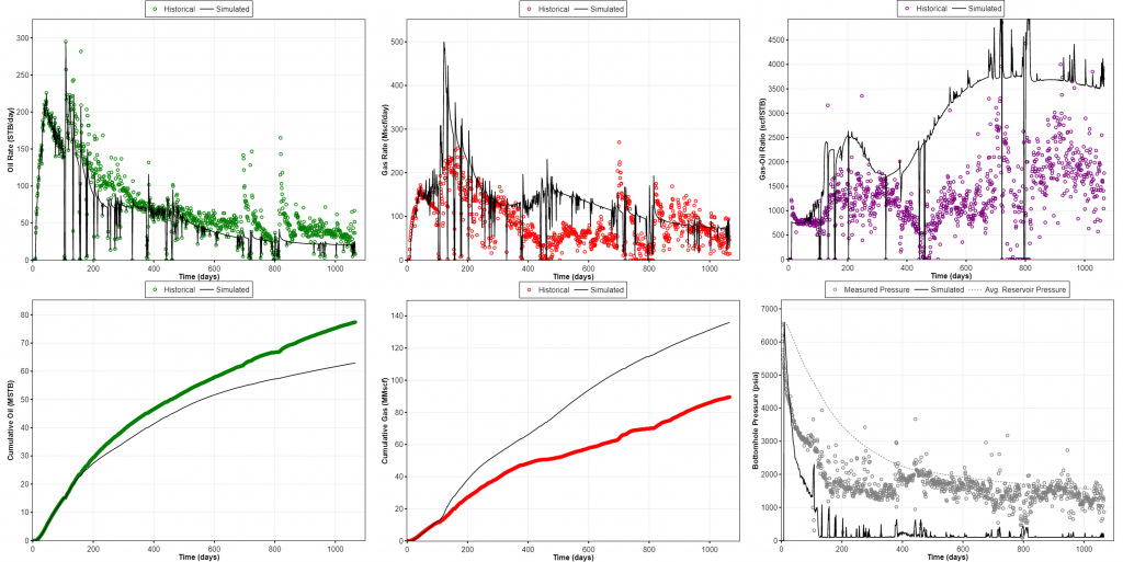
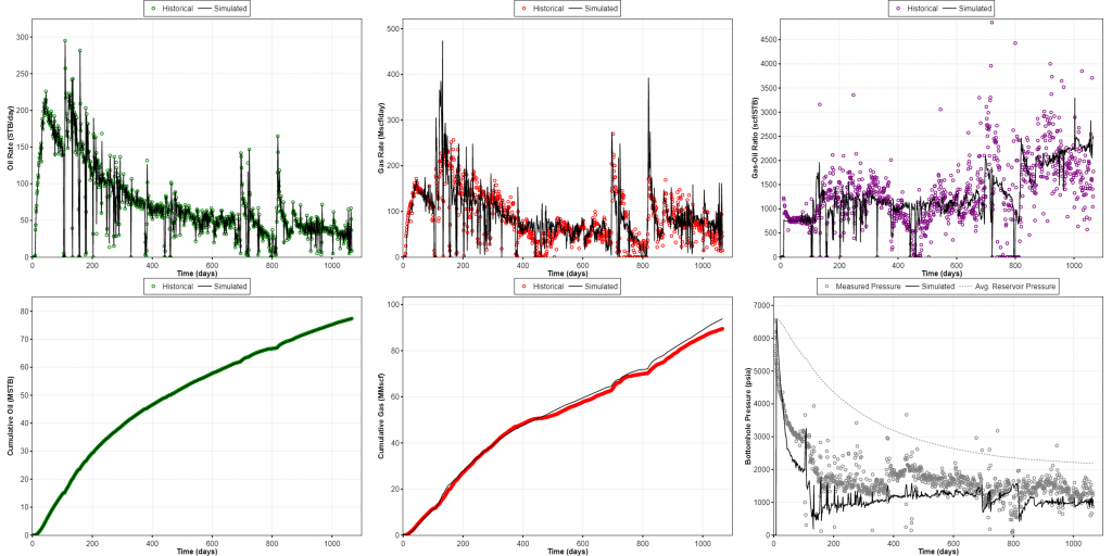
We can see how representative the resulting reservoir property estimates given by the two methods by taking the results into a numerical model and comparing the simulated results with the historical data as seen in Fig. 7 and 8. The results from ARTA give smaller OOIP than the actual model which can be seen from the flowing bottomhole pressure profile that quickly drops to minimum value, and higher GOR than the historical data. The simulated results given by NRTA looks more similar with historical data trend than the ARTA results. Some adjustments may be necessary to improve the quality of history matching results, but for the first run, the NRTA is considered to give a better starting point.

Summary

It is important to understand the underlying assumptions in rate transient analysis (RTA). ARTA, although straightforward, has major problems with multiphase flow and superposition effects. NRTA handles these problems by using a full-physics numerical model. For wells producing with pressure below p_sat, ARTA is still valid if the flow hits the boundary before the pressure reaches p_sat, but this is not possible to know before-hand.

Neither ARTA nor NRTA are guaranteed to predict perfect results, but experience so far points to NRTA being much more reliable than ARTA. We have summarized the main pros and cons of ARTA and NRTA above, but there is one inherent flaw with both methods that needs careful consideration: the engineer’s subjective choice of t_elf in the RNP vs √t plot for ARTA, or the choice of LFP’ stem for NRTA. However, as shown in Bowie and Ewert (2020), there is much less spread or bias in the selected LFP’ compared to t_elf by the test group of engineers, which is another argument for NRTA being a more robust analysis than ARTA.

Misinterpretations can have a negative impact on the future field development & optimization plan. Too short time to end of linear flow yields higher permeability and shorter fracture half-length, which are incorrectly suggest more wells or fewer clusters. It is wise to always verify the results from analytical RTA using numerical RTA which is backed by a full physics numerical simulator.

	Analytical RTA	Numerical RTA
Advantages	Straightforward, no special tool needed	Works for all fluid systems  Accounts for multiphase flow and superposition effects Utilizes a full-physics numerical model
Limitations	Works only for single-phase flow High telf uncertainty (due to multiphase flow and superposition effects)	Require access to a full-physics reservoir simulator (or tool with these capabilities) Require multiple times alterations to inputs (fluid initialization and relative permeability curves) prior analysis

References

Bowie, Braden, and James Ewert. “Numerically Enhanced RTA Workflow – Improving Estimation of Both Linear Flow Parameter And Hydrocarbons In Place.” Paper presented at the SPE/AAPG/SEG Unconventional Resources Technology Conference, Virtual, July 2020. doi: https://doi.org/10.15530/urtec-2020-2967

Carlsen, Mathias Lia, Bowie, Braden, Dahouk, Mohamad Majzoub, Mydland, Stian , Whitson, Curtis Hays, and Ilina Yusra. “Numerical RTA in Tight Unconventionals.” Paper presented at the SPE Annual Technical Conference and Exhibition, Dubai, UAE, September 2021. doi: https://doi.org/10.2118/205884-MS

SPE Data Repository: Data Set: 1, Well Number: 4. From URL: https://www.spe.org/en/industry/data-repository/

Palacio, J.C., and T.A. Blasingame. “Decline-Curve Analysis With Type Curves – Analysis of Gas Well Production Data.” Paper presented at the Low Permeability Reservoirs Symposium, Denver, Colorado, April 1993. doi: https://doi.org/10.2118/25909-MS

Wattenbarger, Robert A., El-Banbi, Ahmed H., Villegas, Mauricio E., and J. Bryan Maggard. “Production Analysis of Linear Flow Into Fractured Tight Gas Wells.” Paper presented at the SPE Rocky Mountain Regional/Low-Permeability Reservoirs Symposium, Denver, Colorado, April 1998. doi: https://doi.org/10.2118/39931-MS

###

Learn more about our consulting capabilities

Global
Curtis Hays Whitson
curtishays@whitson.com

Asia-Pacific
Kameshwar Singh
singh@whitson.com

Middle East
Ahmad Alavian
alavian@whitson.com

Americas
Mathias Lia Carlsen
carlsen@whitson.com

About whitson
whitson supports energy companies, oil services companies, investors and government organizations with expertise and expansive analysis within PVT, gas condensate reservoirs and gas-based EOR. Our coverage ranges from R&D based industry studies to detailed due diligence, transaction or court case projects. We help our clients find the best possible answers to complex questions and assist them in the successful decision-making on technical challenges. We do this through a continuous, transparent dialog with our clients – before, during and after our engagement. The company was founded by Dr. Curtis Hays Whitson in 1988 and is a Norwegian corporation located in Trondheim, Norway, with local presence in USA, Middle East, India and Indonesia