EOS Component Lumping Optimization
To reduce CPU time in compositional petroleum simulation models (e.g. compositional reservoir simulations), a minimum number of components should be used in the equation of state (EOS) to describe the fluid phase and volumetric behavior. A ″detailed” EOS model often contains from 20 to 40 components, with the first 10 components representing pure compounds (H2S , CO2, N2, C1, C2, C3, i-C4, n-C4, i-C5, and n-C5) and the remaining components representing a split of the heavier C6+ material in single-carbon-number (SCN) fractions. A ″pseudoized” (or lumped) EOS model might contain only 6–9 lumped components. Occasionally the light aromatics BTX (benzene, toluene, and xylene isomers) are also kept as separate components for process modeling. Today’s typical laboratory compositional analysis provides 50–60 components, including isomers with carbon numbers 6 to 10, SCN fractions out to C35 and a residual C36+.
On the one hand, lumped EOS models enable engineers to lower considerably the runtime of some discipline-specific applications (e.g. reservoir simulator). On the other hand, the lumping scheme can have major impact on the accuracy of the EOS predictions. This is why finding the optimal EOS lumping scheme is important. For the same number of pseudo-components (i.e. the same runtime in engineering software applications), fluid behavior predictions can be significantly different.
The selection of which components to lump together is difficult because of the huge number of possible combinations. In previous monthly articles, we presented two methods that we have been successfully using at whitson to build lumped EOS models:
- One method consists of a global search of the solution space, see https://whitson.com/2019/10/06/global-component-lumping-for-eos-calculations/
- The other method consists of a genetic algorithm and tabu search algorithm, see https://whitson.com/2020/10/08/eos-component-lumping-optimization/
Both methods can successfully find the optimal EOS lumping scheme that minimizes an objective function. The objective is usually expressed as a RMS measuring the weighted deviation of the lumped EOS model predictions from the original detailed EOS model.
In both methods, pseudo-component properties and BIP’s are internally calculated by the PVT simulator. No extra regression on the pseudo-component properties and BIP’s are added.
Why is it important to match saturation pressures?
Inaccurate saturation pressure predictions can have a strong impact on fluid property predictions, especially for the incipient phase right below the saturation pressure. An under-predicted bubble point pressure leads for example to an over-predicted liquid saturation for pressures below the measured saturation pressure.
The final RMS, which is the objective function of the EOS lumping optimization, is then primarily dominated by the saturation pressure predictions. The effective weight of saturation pressures in the calculation of the RMS is significantly greater than the weights assigned to other PVT data, since a deviation in saturation pressures inevitably leads to a deviation in some other PVT properties (for 2-phase systems). Eventually, this can lead to suboptimal selection of lumping schemes.
A solution to tackle this problem consists of trying to match the saturation pressures each time a new lumping scheme is evaluated. The usual way to match saturation pressures is by multiplying the BIP’s of the lightest pseudo-component (usually, the pseudo-component containing C1) with all the heaviest pseudo-components (usually, the first heavy pseudo-component is the first pseudo-component containing C7) by a single multiplier (usually varying between 0.5 and 1.5). Finding the optimal multiplier that minimizes the discrepancies between measured and predicted saturation pressures requires a regression, leading to increased runtime when evaluating a lumping scheme.
To tune or not to tune?
As an example, we used the 3 cases presented by Alavian et al. (2014): lumping EOS-34 into EOS-15, EOS-9 and EOS-6. For each case, we used the genetic/Tabu search method with three different settings:
- No BIP’s tuning;
- BIP’s tuning on the best lumping scheme only (using a single multiplier as described above);
- BIP’s tuning for every new lumping scheme that is evaluated (using a single multiplier as described above);
and compare the following key performance indicators: optimal lumping schemes, runtime, RMS to try to answer this Shakespearean question: to tune or not to tune?
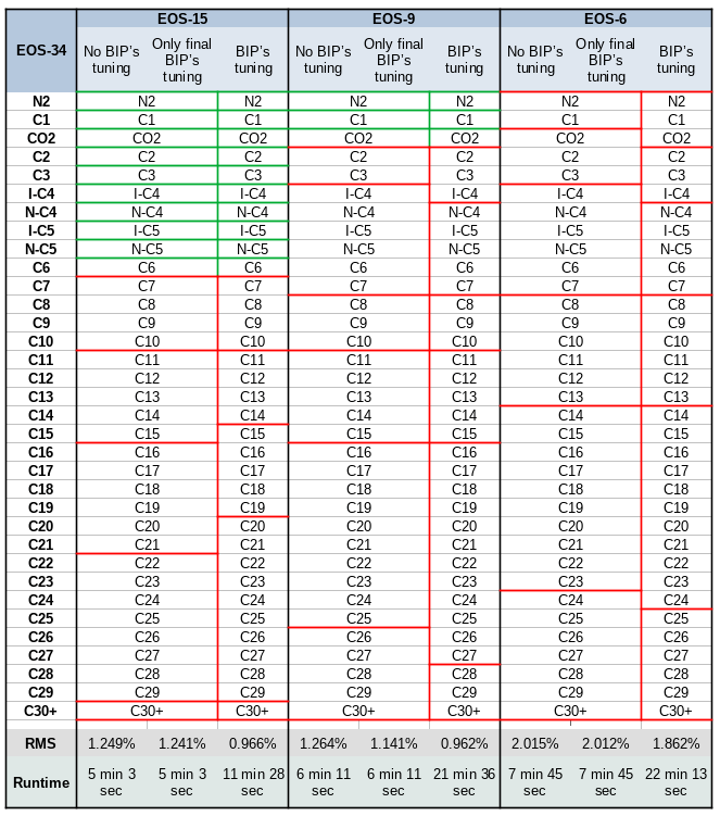
Note that the green pseudo-components are components defined by the user and held constant during the lumping optimization (see Alavian et al.) and the red pseudo-components are obtained by the EOS lumping optimization algorithm.
Conclusions
- Tuning BIP’s during EOS component lumping optimization has a significant impact on the selection of the optimal lumping scheme.
- The gain of tuning BIP’s at every lumping scheme evaluation in terms of RMS ranges from 5 to 25 %, compared to the scenario where BIP’s are not tuned at all. Tuning the BIP’s on the final lumping scheme only leads to a slight improvement (< 1 % ) for the EOS-15 and EOS-6 cases but can also lead to a non-neglectable improvement of the RMS, see the EOS-9 case (± 10 %).
- The runtime increases by a factor 2 to 3, due to the additional BIP’s multiplier regression occuring at every lumping scheme evaluation.
If runtime is not an issue, we strongly advise to tune the BIP’s at every lumping scheme evaluation. It enables the optimization algorithm (especially, neighbor search algorithm like the Tabu search) to explore the solution space more efficiently and ultimately, leads to lumped EOS models that predict phase behavior more accurately.
###
Learn more about our consulting capabilities
Global
Curtis Hays Whitson
curtishays@whitson.com
Asia-Pacific
Kameshwar Singh
singh@whitson.com
Middle East
Ahmad Alavian
alavian@whitson.com
Americas
Mathias Lia Carlsen
carlsen@whitson.com
About whitson
whitson supports energy companies, oil services companies, investors and government organizations with expertise and expansive analysis within PVT, gas condensate reservoirs and gas-based EOR. Our coverage ranges from R&D based industry studies to detailed due diligence, transaction or court case projects. We help our clients find the best possible answers to complex questions and assist them in the successful decision-making on technical challenges. We do this through a continuous, transparent dialog with our clients – before, during and after our engagement. The company was founded by Dr. Curtis Hays Whitson in 1988 and is a Norwegian corporation located in Trondheim, Norway, with local presence in USA, Middle East, India and Indonesia